bmetaweb provides a web interface to the R package bmeta, designed to use Bayesian meta-analytic methods for evidence synthesis.

Meta-analysis is a commonly used statistical approach for evidence synthesis by integrating results from independent studies and is considered to play an essential role in evidence-based medicine. Most applied implementations of meta-analysis are conducted under the Frequentist paradigm. However, it is often the case that using a Bayesian approach can be beneficial in the context of meta-analysis. The main advantages are that Bayesian methods allow to include a formal representation of prior belief in the model and uncertainties related to both parameters and model can be better accounted for. The bmetaweb is easy and straightforward to use. First, users need to specify a Bayesian meta-analytic model to fit the observed data. The types of outcomes for selection include binary, continuous and count and then, users need to decide whether to use a meta-analysis or a meta-regression accounting for moderator effects and specify the type of models (i.e. fixed- or random-effects model) to be performed. Finally, users can select the prior to be included in the model designed for a specific type of outcome. And these are the pre-steps required by bmeta and bmetaweb before automatically performing the analysis and producing standardised output based on the Bayesian meta-analytic methods. In addition, bmetaweb can also save the model template selected by the user. These templates can be modified easily to fit other scenarios or saved for future reference.

bmetaweb assumes that the studies included only have two arms comparing a single intervention and users must provide essential information of the two arms for comparison. For example, for the binary data, users must provide the sample size of both case and control arm and the events observed in the two arms. If meta-regression models are selected, users need to pay special attention to the format of covariates which are categorical and this includes specifying a baseline category and stratify each of the rest categories into dummy variables. For example, if different studies report using population of distinct ethnic groups---White, Black, Asian. Then users need to select a baseline group, suppose we use Asian here, and then for White and Black, dummy variables need to be created to indicate whether the study used a certain ethnic group or not. Therefore, in this case, in this meta-regression model, two covariates need to be used, each representing the incremental effects of ethnicity in comparion to the baseline group (Asian). These observed data need to be formatted properly and uploaded by the user in MS Excel formats: a spreadsheet in.csv format, e.g. a file produced by MS Excel. Download an example here .

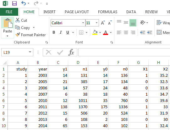
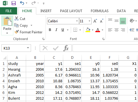
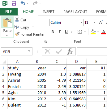
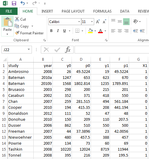
The observed data are uploaded at the 'Load data and model selection' tab. Once the user specifies a desired model and uploads the spreadsheet, the analysis will be automatically run. bmetaweb assumes that the user has saved all the observed data in an appropriate manner for each of the studies being assessed in a .csv file. The variables in this file need to be like in the following pictures. The first picture presents the spreadsheet template for binary data (i.e. y1 and y0: number of events in case and control arm; n1 and n0: total sample size of case and control arm). The next two pictures show the template for continuous data as it is assumed that there are two types of studies. The first type of study provides detailed information of both case and control arm (i.e. y1 and y0: mean of the case and control arm; se1 and se0: standard error of case and control arm) whereas the second type of study only report mean difference between the two arm (y) and the variance (var). Notice that the variance is computed as the sum of variances of the two arms. The last graph illustrates the template for count data (y1 and y0: total number of events in the follow-up period for case and control arm; p1 and p0: total follow-up person years---computed as the total number of patients times the total number of follow-up time). It should also be noted that users need to save the covariates (i.e. X1, X2,...,Xj) starting from the 7th column except for the second type of continuous data (studies reporting mean difference between the two arms and the variance) where covariates start from the 5th column. The study characteristics such as author name and year of publication need to be named as 'study' and 'year' (notice the first letter of these variable names is not capital).






An example of such a file can be obtained here. After specifying the desired meta-analytic model in the 'Load data and model selection' tab, this spreadsheet can be uploaded and the model will run bmeta in the background and create all the relevant output summaries. The output table will appear in the right panel and users can further specify the plots to visualise the outcomes. In addition, some diagnostic plots are available to assess the model fit and performance by clicking the 'Diagnostics' tab. The results of the Bayesian meta-analystic models performed using bmetaweb can be exported in either .pdf or .doc format. The resulting report contains some pre-formatted text, aimed at guiding the user through the interpretation of the results.


Copyright: Tao Ding, Gianluca Baio